Run an i-vector system
This script runs an experiment on the male NIST Speaker Recognition Evaluation 2010 extended core task. For more details about the protocol, refer to the NIST-SRE website.
In order to get this scirpt running on your machine, you will need to modify a limited number of options to indicate where your features are located and how many threads you want to run in parallel.
Getting ready
Load your favorite modules before going further.
import sidekit
Set parameters of your system:
distrib_nb = 2048  # number of Gaussian distributions for each GMM
rank_TV = 400  # Rank of the total variability matrix
tv_iteration = 10  # number of iterations to run
plda_rk = 400  # rank of the PLDA eigenvoice matrix
feature_dir = '/lium/spk1/larcher/mfcc_24/'  # directory where to find the features
feature_extension = 'h5'  # Extension of the feature files
nbThread = 10  # Number of parallel process to run
Load list of files to process. All the files neede to run this tutorial are available at Download lists for standard datasets.
with open("task/ubm_list.txt", "r") as fh:
    ubm_list = np.array([line.rstrip() for line in fh])
tv_idmap = sidekit.IdMap("task/tv_idmap.h5")
plda_male_idmap = sidekit.IdMap("task/plda_male_idmap.h5")
enroll_idmap = sidekit.IdMap("task/core_male_sre10_trn.h5")
test_idmap = sidekit.IdMap("task/test_sre10_idmap.h5")
The lists needed are:
the list of files to train the GMM-UBM
an IdMap listing the files to train the total variability matrix
an IdMap to train the PLDA, WCCN, Mahalanobis matrices
the IdMap listing the enrolment segments and models
the IdMap describing the test segments
Load Key and Ndx:
test_ndx = sidekit.Ndx("task/core_core_all_sre10_ndx.h5")
keys = sidekit.Key('task/core_core_all_sre10_cond5_key.h5')
Define the FeaturesServer to load the acoustic features:
fs = sidekit.FeaturesServer(feature_filename_structure="{dir}/{{}}.{ext}".format(dir=feature_dir, ext=feature_extension),
                            dataset_list=["energy", "cep", "vad"],
                            mask="[0-12]",
                            feat_norm="cmvn",
                            keep_all_features=False,
                            delta=True,
                            double_delta=True,
                            rasta=True,
                            context=None)
Train your system
Train now the UBM-GMM using EM algorithm and write it to disk. After each iteration, the current version of the mixture is written to disk.
ubm = sidekit.Mixture()
llk = ubm.EM_split(fs, ubm_list, distrib_nb, num_thread=nbThread, save_partial='gmm/ubm')
ubm.write('gmm/ubm_{}.h5'.format(distrib_nb))
Create StatServers for the enrollment, test and background data and compute the statistics:
enroll_stat = sidekit.StatServer(enroll_idmap, ubm)
enroll_stat.accumulate_stat(ubm=ubm, feature_server=fs, seg_indices=range(enroll_stat.segset.shape[0]) ,num_thread=nbThread)
enroll_stat.write('data/stat_sre10_core-core_enroll_{}.h5'.format(distrib_nb))

test_stat = sidekit.StatServer(test_idmap, ubm)
test_stat.accumulate_stat(ubm=ubm, feature_server=fs, seg_indices=range(test_stat.segset.shape[0]), num_thread=nbThread)
test_stat.write('data/stat_sre10_core-core_test_{}.h5'.format(distrib_nb))

back_idmap = plda_all_idmap.merge(tv_idmap)
back_stat = sidekit.StatServer(back_idmap, ubm)
back_stat.accumulate_stat(ubm=ubm, feature_server=fs, seg_indices=range(back_stat.segset.shape[0]), num_thread=nbThread)
back_stat.write('data/stat_back_{}.h5'.format(distrib_nb))
Train Total Variability Matrix for i-vector extraction. After each iteration, the matrix is saved to disk.
tv_stat = sidekit.StatServer.read_subset('data/stat_back_{}.h5'.format(distrib_nb), tv_idmap)
tv_mean, tv, _, __, tv_sigma = tv_stat.factor_analysis(rank_f = rank_TV,
                                                       rank_g = 0,
                                                       rank_h = None,
                                                       re_estimate_residual = False,
                                                       it_nb = (tv_iteration,0,0),
                                                       min_div = True,
                                                       ubm = ubm,
                                                       batch_size = 100,
                                                       num_thread = nbThread,
                                                       save_partial = "data/TV_{}".format(distrib_nb))
sidekit.sidekit_io.write_tv_hdf5((tv, tv_mean, tv_sigma), "data/TV_{}".format(distrib_nb))
Extract i-vectors for target models, training and test segments:
enroll_stat = sidekit.StatServer('data/stat_sre10_core-core_enroll_{}.h5'.format(distrib_nb))
enroll_iv = enroll_stat.estimate_hidden(tv_mean, tv_sigma, V=tv, batch_size=100, num_thread=nbThread)[0]
enroll_iv.write('data/iv_sre10_core-core_enroll_{}.h5'.format(distrib_nb))

test_stat = sidekit.StatServer('data/stat_sre10_core-core_test_{}.h5'.format(distrib_nb))
test_iv = test_stat.estimate_hidden(tv_mean, tv_sigma, V=tv, batch_size=100, num_thread=nbThread)[0]
test_iv.write('data/iv_sre10_core-core_test_{}.h5'.format(distrib_nb))

plda_stat = sidekit.StatServer.read_subset('data/stat_back_{}.h5'.format(distrib_nb), plda_all_idmap)
plda_iv = plda_stat.estimate_hidden(tv_mean, tv_sigma, V=tv, batch_size=100, num_thread=nbThread)[0]
plda_iv.write('data/iv_plda_{}.h5'.format(distrib_nb))
Run the tests
keys = []
for cond in range(9):
    keys.append(sidekit.Key('/lium/buster1/larcher/nist/sre10/core_core_{}_sre10_cond{}_key.h5'.format("all", cond + 1)))

enroll_iv = sidekit.StatServer('data/iv_sre10_core-core_enroll_{}.h5'.format(distrib_nb))
test_iv = sidekit.StatServer('data/iv_sre10_core-core_test_{}.h5'.format(distrib_nb))
plda_iv = sidekit.StatServer.read_subset('data/iv_plda_{}.h5'.format(distrib_nb), plda_male_idmap)
Using Cosine similarity
A simple cosine scoring without any normalization of the i-vectors.
scores_cos = sidekit.iv_scoring.cosine_scoring(enroll_iv, test_iv, test_ndx, wccn = None)
A version where i-vectors are normalized using Within Class Covariance normalization (WCCN).
wccn = plda_iv.get_wccn_choleski_stat1()
scores_cos_wccn = sidekit.iv_scoring.cosine_scoring(enroll_iv, test_iv, test_ndx, wccn=wccn)
The same with a Linear Discriminant Analysis performed first to reduce the dimension of i-vectors to 150 dimensions.
LDA = plda_iv.get_lda_matrix_stat1(150)

plda_iv_lda = copy.deepcopy(plda_iv)
enroll_iv_lda = copy.deepcopy(enroll_iv)
test_iv_lda = copy.deepcopy(test_iv)

plda_iv_lda.rotate_stat1(LDA)
enroll_iv_lda.rotate_stat1(LDA)
test_iv_lda.rotate_stat1(LDA)

scores_cos_lda = sidekit.iv_scoring.cosine_scoring(enroll_iv_lda, test_iv_lda, test_ndx, wccn=None)
And now combine LDA and WCCN:
wccn = plda_iv_lda.get_wccn_choleski_stat1()
scores_cos_lda_wcnn = sidekit.iv_scoring.cosine_scoring(enroll_iv_lda, test_iv_lda, test_ndx, wccn=wccn)
Using Mahalanobis distance
If the scoring is ‘mahalanobis’, i-vectors are normalized using one iteration of the Eigen Factor Radial algorithm (equivalent to the so called length-normalization). Then scores are computed using a Mahalanobis distance.
meanEFR, CovEFR = plda_iv.estimate_spectral_norm_stat1(3)

plda_iv_efr1 = copy.deepcopy(plda_iv)
enroll_iv_efr1 = copy.deepcopy(enroll_iv)
test_iv_efr1 = copy.deepcopy(test_iv)

plda_iv_efr1.spectral_norm_stat1(meanEFR[:1], CovEFR[:1])
enroll_iv_efr1.spectral_norm_stat1(meanEFR[:1], CovEFR[:1])
test_iv_efr1.spectral_norm_stat1(meanEFR[:1], CovEFR[:1])
M1 = plda_iv_efr1.get_mahalanobis_matrix_stat1()
scores_mah_efr1 = sidekit.iv_scoring.mahalanobis_scoring(enroll_iv_efr1, test_iv_efr1, test_ndx, M1)
Using Two-covariance scoring
If the scoring is ‘2cov’, two 2-covariance models are trained with and without i-vector normalization. The normalization applied consists of one iteration of Spherical Noramlization.
W = plda_iv.get_within_covariance_stat1()
B = plda_iv.get_between_covariance_stat1()
scores_2cov = sidekit.iv_scoring.two_covariance_scoring(enroll_iv, test_iv, test_ndx, W, B)

meanSN, CovSN = plda_iv.estimate_spectral_norm_stat1(1, 'sphNorm')

plda_iv_sn1 = copy.deepcopy(plda_iv)
enroll_iv_sn1 = copy.deepcopy(enroll_iv)
test_iv_sn1 = copy.deepcopy(test_iv)

plda_iv_sn1.spectral_norm_stat1(meanSN[:1], CovSN[:1])
enroll_iv_sn1.spectral_norm_stat1(meanSN[:1], CovSN[:1])
test_iv_sn1.spectral_norm_stat1(meanSN[:1], CovSN[:1])

W1 = plda_iv_sn1.get_within_covariance_stat1()
B1 = plda_iv_sn1.get_between_covariance_stat1()
scores_2cov_sn1 = sidekit.iv_scoring.two_covariance_scoring(enroll_iv_sn1, test_iv_sn1, test_ndx, W1, B1)
Using Probabilistic Linear Discriminant Analysis
Normalize i-vector using Spherical Nuisance Normalization and compute scores using Probabilistic Linear Discriminant Analysis
meanSN, CovSN = plda_iv.estimate_spectral_norm_stat1(1, 'sphNorm')

plda_iv.spectral_norm_stat1(meanSN[:1], CovSN[:1])
enroll_iv.spectral_norm_stat1(meanSN[:1], CovSN[:1])
test_iv.spectral_norm_stat1(meanSN[:1], CovSN[:1])

plda_mean, plda_F, plda_G, plda_H, plda_Sigma = plda_iv.factor_analysis(rank_f=plda_rk,
                                                                        rank_g=0,
                                                                        rank_h=None,
                                                                        re_estimate_residual=True,
                                                                        it_nb=(10,0,0),
                                                                        min_div=True,
                                                                        ubm=None,
                                                                        batch_size=1000,
                                                                        num_thread=nbThread)

sidekit.sidekit_io.write_plda_hdf5((plda_mean, plda_F, plda_G, plda_Sigma), "data/plda_model_tel_m_{}.h5".format(distrib_nb))

scores_plda = sidekit.iv_scoring.PLDA_scoring(enroll_iv, test_iv, test_ndx, plda_mean, plda_F, plda_G, plda_Sigma, full_model=False)
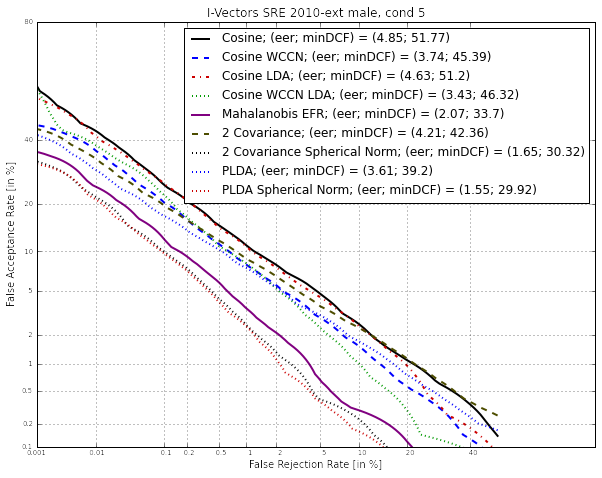
Plot the DET curves
In case you want to display the results of the experiments. First define the target prior, the parameters of the graphic window and the title of the plot.
# Set the prior following NIST-SRE 2010 settings
prior = sidekit.logit_effective_prior(0.001, 1, 1)
# Initialize the DET plot to 2010 settings
dp = sidekit.DetPlot(windowStyle='sre10', plotTitle='I-Vectors SRE 2010-ext male, cond 5')
For each of the performed experiments, load the target and non-target scores for the condition 5 according to the key file.
dp.set_system_from_scores(scores_cos, keys, sys_name='Cosine')
dp.set_system_from_scores(scores_cos_wccn, keys, sys_name='Cosine WCCN')
dp.set_system_from_scores(scores_cos_lda, keys, sys_name='Cosine LDA')
dp.set_system_from_scores(scores_cos_wccn_lda, keys, sys_name='Cosine WCCN LDA')

dp.set_system_from_scores(scores_mah_efr1, keys, sys_name='Mahalanobis EFR')

dp.set_system_from_scores(scores_2cov, keys, sys_name='2 Covariance')
dp.set_system_from_scores(scores_2cov_sn1, keys, sys_name='2 Covariance Spherical Norm')

dp.set_system_from_scores(scores_plda, keys, sys_name='PLDA')
Create the window and plot:
dp.create_figure()
dp.plot_rocch_det(0)
dp.plot_rocch_det(1)
dp.plot_rocch_det(2)
dp.plot_rocch_det(3)
dp.plot_rocch_det(4)
dp.plot_rocch_det(5)
dp.plot_rocch_det(6)
dp.plot_rocch_det(7)
dp.plot_DR30_both(idx=0)
dp.plot_mindcf_point(prior, idx=0)
Depending of the data available, the following plot could be obtained at the end of this tutorial: (For this example, data used include NIST-SRE 04, 05, 06, 08, the SwitchBoard Part 2 phase 2 and 3 and Cellular part 2) Those results are far from optimal as don’t generalize on other conditions of NIST-SRE 2010. This system has been trained without any specific data selection and its purpose is only to give an idea of what you can obtain.